Learning Center

How to build a forecast model?

SAFE TOOLBOXES^® comes with the following forecast models:

Regression models can also be used for forecasting purposes. This can be done separating one part of your data to represent the “past” and another part of your data to represent the “future”. This method may be useful if the explanatory variables are known in advance or if they are easier to predicted than the dependent variable itself. In this approach only the “past” portion of your data is used to fit the parameters of the regression model.

A short example

Consider the following time series:

	A	B	C
1	Sample database
2
3	Time	Value
4	1	103.2
5	2	106.6
6	3	106.6
7	4	106.6
8	5	106.6
9	6	106.6
10	7	108.5
11	8	111.7
12	9	116.2
13	10	117.4
14	11	119.2
15	12	121.0
16	13	122.5
17	14	124.2
18	15	119.1
19	16	117.0
20	17	114.0
21	18	109.0
22	19	107.0
23	20	104.0
24	21	98.2
25	22	93.5
26	23	88.7
27	24	83.9
28	25	80.7
29	26	78.5
30	27	73.9
31	28	72.3
32	29	71.4
33	30	71.6
34	31	71.1
35	32	71.2
36	33	71.5
37	34	72.6
38	35	74.2
39	36	79.0
40	37	82.3
41	38	84.5
42	39	89.0
43	40	92.5
44	41	94.5
45	42	99.0
46	43	101.7
47	44	104.3
48	45	106.5
49	46	108.7
50	47	109.0
51	48	109.0
52	49	109.0
53	50	109.0
54

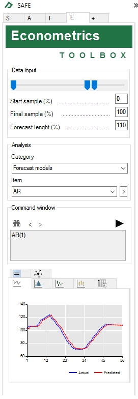
To forecast a value for dates 51 to 55 of this series using an AR(1) model just follow the steps below:

1. Select the Econometrics Toolbox tab
2. Select any cell containing the series (let’s say, cell B5)
3. Adjust the start sample to 0% and the final sample to 100% (to use all 50 sample points) and the forecast length to 110% (to predict inside the sample and five extras points)
4. Set option Category = “Forecast models” and item = “AR” under the "Analysis" group and click on the button to confirm your choice
5. Specify the order of the AR model changing the text “AR(p)” to “AR(1)” in the command window textbox and click on the button

Now, the results will appear at the bottom of the Econometrics Toolbox tab.

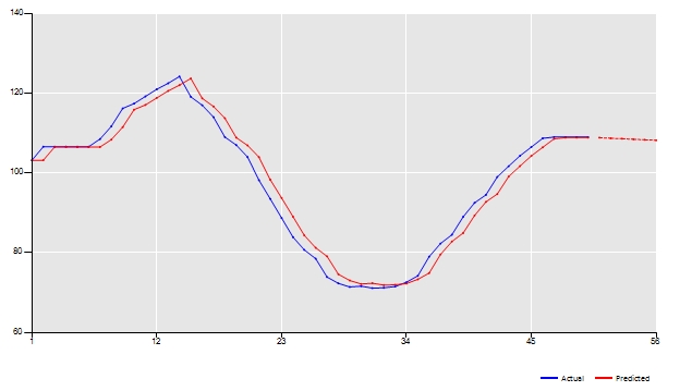
A first check of the goodness of fit of our model can be done by inspecting the line plot chart. A good fit will put the red line (predicted values) near to the blue line (actual values). The dotted line represents the out of sample prediction of our model.

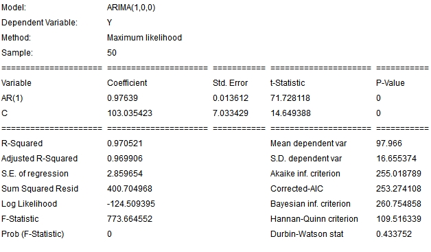
The equation of our AR(1) model is placed in the tab. This table shows the fitted parameters and useful statistics of our model. Not all forecasting models have a representation in the equation tab. This is the case, for instance, for the Holt-Winters models or the moving average model.

You can run different specification for your ARIMA model or use other forecast methodologies. The “Historical results” tab will keep the main statistics of your models. Particularly, in the case of forecasting models, is a good practice to reserve some portion of your data to run out of sample tests. By doing this, the forecast statistics: MAD (mean absolute deviation), MAPE (mean absolute percent error) and RMSE (root of mean square error) available in this tab can help you to rank your models.