Learning Center
How to run a Monte Carlo simulation?
In this article we are going to cover these four different methods to run a Monte Carlo simulation within Excel:
- Method 1
- Simple Monte Carlo simulation
- Method 2
- Monte Carlo simulation by the iterative calculus trick
- Method 3
- Monte Carlo simulation by the data table trick
- Method 4
- Monte Carlo simulation using SAFE TOOLBOXES®
The first three of them could be done using only Excel, and the last one shows how to run a simulation with SAFE TOOLBOXES®. So, if you are only interested in how to run a Monte Carlo using SAFE TOOLBOXES®, you can go straight to the last method.
Method 1: Simple Monte Carlo simulation
Running a Monte Carlo Simulation is a very simple procedure and for the univariate case it consists only in: a) Sample a number "x" from a uniform distribution; and b) transform this number in the desired distribution using the inverse function y= f-1(x).
So, for instance, to draw a sample from a standard normal distribution, simply enter a formula in the spreadsheet like:
A |
B |
C |
D |
E |
F |
|
1 |
Sample from standard normal distribution: |
0.33 |
=NORMSINV(RAND()) |
|
|
|
2 |
|
|
|
|
|
|
and then press F9 to get one more sample.
The disadvantage of this technique is that it does not keep the results from one round of calculation to the other (that is, each time that you press F9 the previous result is discarded), so the only way to get the summary stats is to replicate the calculus in some other cells in order to have multiple samples at the same time of the calculation. This can be very cumbersome if there is a complex chain of dependency between random variables in the spreadsheet.
The simulation for the multivariate case is very similar to the univariate case and some additional steps are necessary to replicate the relationship among variables, using, for instance, the Cholesky decomposition of the correlation or covariance matrix or for more complex dependencies the Copula technique to simulate multivariate random variables.
Method 2: Monte Carlo simulation by iterative calculus trick
This approach goes one step forward from the previous one by turning on the iterative calculation in the Excel options. By using this method it is possible to recover from any cell that has a random value: a) the variable sample average, and b) the variable variance/standard deviation.
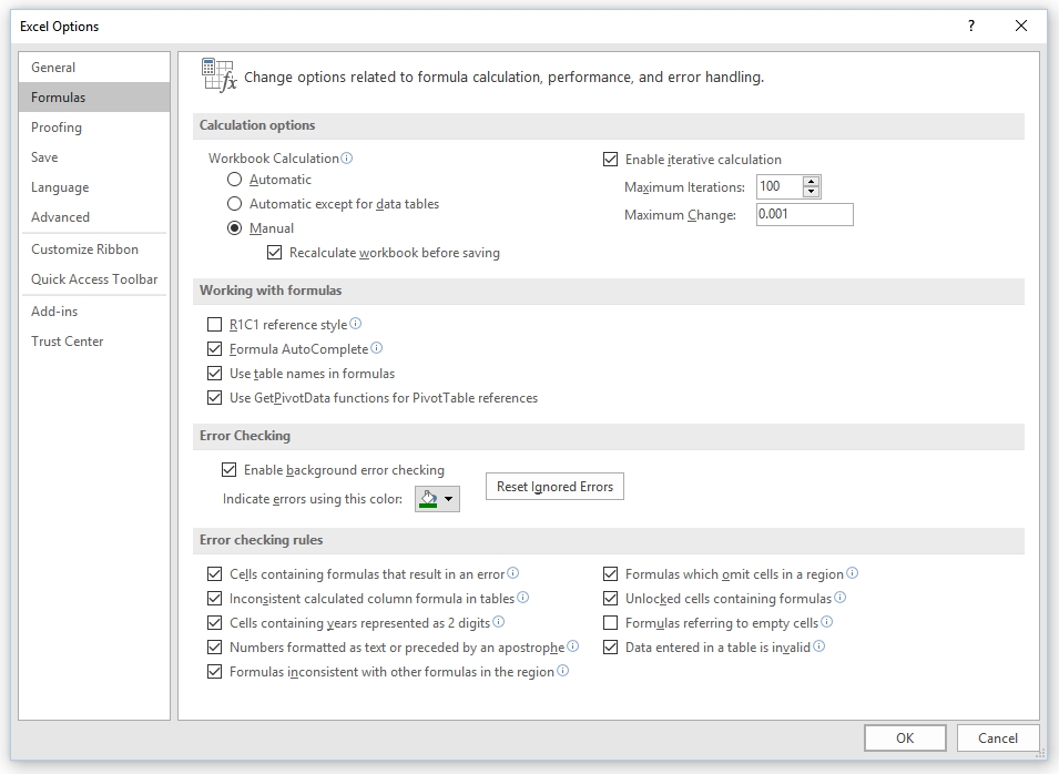
Let’s first do the trick before entering in some details on how it works. First of all, after configuring a random variable, go to the Excel options and check the box “Enable iterative calculation”, change the calculation to manual and then define the number of desired simulations in the field “Maximum iterations”.
Then, write these formulas in the cells A1:B7:
A |
B |
C |
D |
E |
|
1 |
Random variable: |
- 0.49 |
=NORMSINV(RAND())+B2*0 |
|
|
2 |
Iteration number: |
1,001.00 |
=B2+1 |
|
|
3 |
Sum of the variable: |
15.90 |
=B3+B1 |
|
|
4 |
Mean: |
0.02 |
=B3/B2 |
|
|
5 |
Variable squared: |
0.24 |
=B1^2 |
|
|
6 |
Sum of the variable squared: |
1,027.96 |
=B6+B5 |
|
|
7 |
Standard deviation: |
1.01 |
=((B6-2*B4*B3+B2*B4^2)/(B2-1))^0.5 |
|
|
Some cells will refuse to be recalculated in each iteration. To overcome this and force them to be recalculated just sum a term like “+ B2*0” at the end of the formula.
Now, each time that you press F9 the specified number of simulations will occur and the running average and standard deviation will be displayed in cells B4 and B7.To restart the counter of iterations and the values of the cells, just select the cell, go to the formula editor and press ENTER.
The magic of this trick is that allowing the iterative calculus in Excel the limitation of circular reference is disabled and referencing a cell to itself allows using the previous value of the cell in the current calculation. Nevertheless, it’s not possible to recover the historical simulated values to be used in other kinds of analysis.
Method 3: Monte Carlo simulation by the data table trick
The primary goal of this method is to perform a Monte Carlo simulation and store every value sampled. The example below shows the logic of the procedure. First, enter the formulas and values displayed below in a new spreadsheet.
A |
B |
C |
D |
E |
|
1 |
Random variable: |
- 1.02 |
=NORMSINV(RAND())+B2*0 |
|
|
2 |
Number to force recalculation: |
0.89 |
=RAND() |
|
|
3 |
|
- 1.02 |
=B1 |
|
|
4 |
1 |
|
|
|
|
5 |
2 |
|
|
|
|
6 |
3 |
|
|
|
|
7 |
4 |
|
|
|
|
8 |
5 |
|
|
|
|
Select the range A3:B8, go to Data > What-if analysis > Data table… and in the form that will open type the text as seen in the figure:
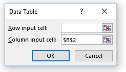
Now, the range B4:B8 will present five samples of the random variable given in B1. Of course, to extend the number of simulations is just a matter of increasing the size of the data table.
The data tables are generally used to analyze the effects of changes in the inputs of some function using the values given in the column of the data table. In this case, we changed the data in an irrelevant fashion just to collect new values of the random function.
The main drawback of this methodology is that data tables are computing intensive and can slow down the Excel spreadsheet.
Method 4: Monte Carlo simulation using SAFE TOOLBOXES®
We are very glad if one of the three methods presented above was enough for the task that you are trying to accomplish. Nevertheless, if you want to save yourself some time and gain access to a complete framework to perform and analyze the results of a Monte Carlo simulation, our software is the right tool that you are looking for.
Besides providing a full range of facilities for entering models that contain random variables, SAFE TOOLBOXES® gives you an instant predefined analysis of the simulations presenting the results as histograms, convergence plots, time series plots, summary statistics and much more.
To give a very introductory example on how to run a Monte Carlo simulation using SAFE, enter the following formula in a new spreadsheet:
A |
B |
C |
D |
E |
|
1 |
Random variable: |
1.02 |
=sRAND_StandardNormal() |
|
|
2 |
|
|
|
|
|
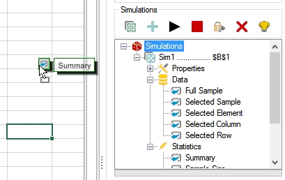
Select the cell B1, click on the button “Simulate” and type the desired number of simulations. That is it! The results will automatically appear in the task pane.
Simulate button
 (Ribbon version) or
 ![]() (Simulation Toolbox tab version)
(Simulation Toolbox tab version)
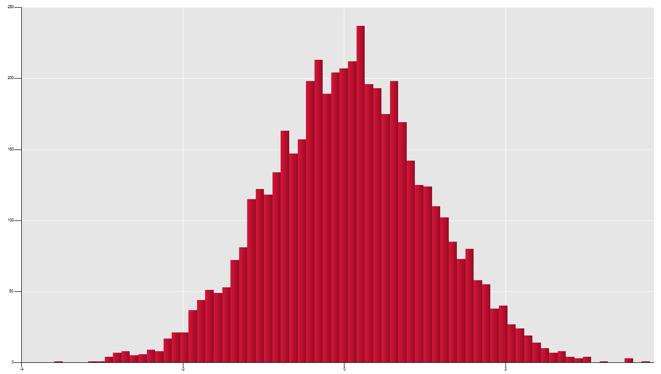
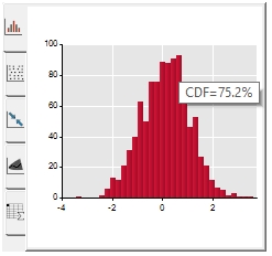
At the bottom of the task pane, the first graph will present the histogram of the simulation. You can also interact with it hovering the mouse over the bars to see the cumulative probability at the selected point. You can also double-click on it to open an enlarged view of the chart.
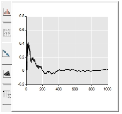
By clicking on the tab ![]() at the bottom at the simulation task pane you will see the running average of the simulation. This information is very useful to check how long the simulation takes to converge to a given value. You can, later on, repeat the simulation using some other methodologies such as the variance reduction technique or pseudo-random numbers to see if there will be some improvement on the convergence.
at the bottom at the simulation task pane you will see the running average of the simulation. This information is very useful to check how long the simulation takes to converge to a given value. You can, later on, repeat the simulation using some other methodologies such as the variance reduction technique or pseudo-random numbers to see if there will be some improvement on the convergence.
The main statistics of the simulation can be seen on the tab ![]() . The summary presents the following stats: sample size, mean, standard deviation, skewness, kurtosis, minimum, 1st quartile, median, 3rd quartile, maximum and the Anderson-Darling and Jarque-Bera normality tests.
. The summary presents the following stats: sample size, mean, standard deviation, skewness, kurtosis, minimum, 1st quartile, median, 3rd quartile, maximum and the Anderson-Darling and Jarque-Bera normality tests.
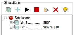
It’s important to notice that you can enter more than one cell to be recorded during the simulation. You can select a continuous range of the spreadsheet, click on the button "add" ![]() and a new simulation will appear in the tree view.
and a new simulation will appear in the tree view.
You can also execute the same procedure to add other ranges of the spreadsheet to be monitored. Every time that you click on the button to simulate all selected ranges that were added will have their values recorded. But, if you want to prevent some simulation object to restart recording in a new round of simulation, just click on the button lock ![]() .
.
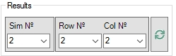
The results of the simulations can be seen selecting the correspondent number of simulation that contains the range, the relative row number of the target cell in the range, and the corresponding column number of the target cell in the range. For instance, suppose that you have added the range “A1:B2” to the “Sim1” and the range “C1:D2” to the “Sim2”. To analyze the simulation of the cell “D2”, enter this selection in the input boxes at the bottom of the tab:
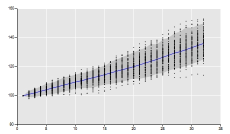
In some cases, the area will represent random time series vectors. With that in mind, the chart![]() plots this vector in a very meaningful fashion. In this chart, the blue line represents the mean of each cell and the gray area represents the interval between the percentiles 5% and 95%.
plots this vector in a very meaningful fashion. In this chart, the blue line represents the mean of each cell and the gray area represents the interval between the percentiles 5% and 95%.
Besides the predefined analysis that follows every simulation, a plenty of spreadsheet functions is available to facilitate working with the results. Most of these functions can be inserted just expanding the tree view of the selected simulation and then dragging and dropping the desired output on the spreadsheet.