Learning Center
How to directly transform a time series?
A direct transformation of a time series can help you exploring your data and creating econometrics models in a blink of an eye. This is because you can use any variation of a time series in your model without having to insert the transformed time series in the spreadsheet. The list of transformations available in the Econometrics Toolbox is:
Exp |
2nd_Difference |
Power(n) |
Log |
Returns |
Fitted_AR(p) |
Sqrt |
AccumulatedReturns |
Fitted_MA(q) |
Normalization |
LogReturns |
Fitted_ARIMA(p,d,q) |
Abs |
AccumulatedLogReturns |
EWMA(lambda) |
Lag |
Square |
Fitted_Garch(p,q) |
Seasonal_Difference |
Series-Mean_Squared |
Error |
1st_Difference |
|
|
Using a transformation in your time series is just a matter of enclosing the transformation in the variable operators (Y[], X1[], X2[], … ) . Multiple operators are allowed, just type the transformations followed by a semicolon. Evaluations are made from the left to the right. So, for instance, Y[power(2); exp] will first apply the function f(x) = x^2 to every data x of the series denoted by Y and then apply the function g(f(x)) = exp(f(x)). As you can note, transformations that contain parenthesis need to have the letters enclosed replaced by appropriate parameters.
There is also one special transformation, the “error” transformation. This transformation returns the difference between the original series and the subsequent transformations until its evocation. Therefore, a transformation like Y[power(2); error] returns a transformed series Z = Y - Y^2, where Y is the original series in the spreadsheet.
All transformations are also available through the function “sTimeSeriesTransform” where you can simply type a transformation string — ex: “Y[log;power(2)]” — as one of the function's arguments.
To practice the above concepts a little bit, we are going to build a transformation to explore how the volatility of the following time series of some stock prices behaves, considering the series below:
A |
B |
C |
D |
E |
F |
|
1 |
Apple Inc. (Adjusted close price) |
|
|
|
|
|
2 |
|
|
|
|
|
|
3 |
2012-12-31 |
71.03051 |
|
|
|
|
4 |
2013-01-02 |
73.28087 |
|
|
|
|
5 |
2013-01-03 |
72.3559 |
|
|
|
|
6 |
2013-01-04 |
70.34045 |
|
|
|
|
7 |
2013-01-07 |
69.92669 |
|
|
|
|
8 |
2013-01-08 |
70.11489 |
|
|
|
|
9 |
2013-01-09 |
69.01907 |
|
|
|
|
10 |
2013-01-10 |
69.87463 |
|
|
|
|
11 |
2013-01-11 |
69.44619 |
|
|
|
|
12 |
2013-01-14 |
66.97025 |
|
|
|
|
13 |
2013-01-15 |
64.85737 |
|
|
|
|
14 |
2013-01-16 |
67.54952 |
|
|
|
|
... |
... |
... |
|
|
|
|
746 |
2015-12-11 |
112.5692 |
|
|
|
|
747 |
2015-12-14 |
111.873 |
|
|
|
|
748 |
2015-12-15 |
109.8937 |
|
|
|
|
749 |
2015-12-16 |
110.7391 |
|
|
|
|
750 |
2015-12-17 |
108.3918 |
|
|
|
|
751 |
2015-12-18 |
105.4578 |
|
|
|
|
752 |
2015-12-21 |
106.7507 |
|
|
|
|
753 |
2015-12-22 |
106.6513 |
|
|
|
|
754 |
2015-12-23 |
108.0238 |
|
|
|
|
755 |
2015-12-24 |
107.447 |
|
|
|
|
756 |
2015-12-28 |
106.2435 |
|
|
|
|
757 |
2015-12-29 |
108.1531 |
|
|
|
|
758 |
2015-12-30 |
106.7408 |
|
|
|
|
759 |
2015-12-31 |
104.6919 |
|
|
|
|
760 |
|
|
|
|
|
|
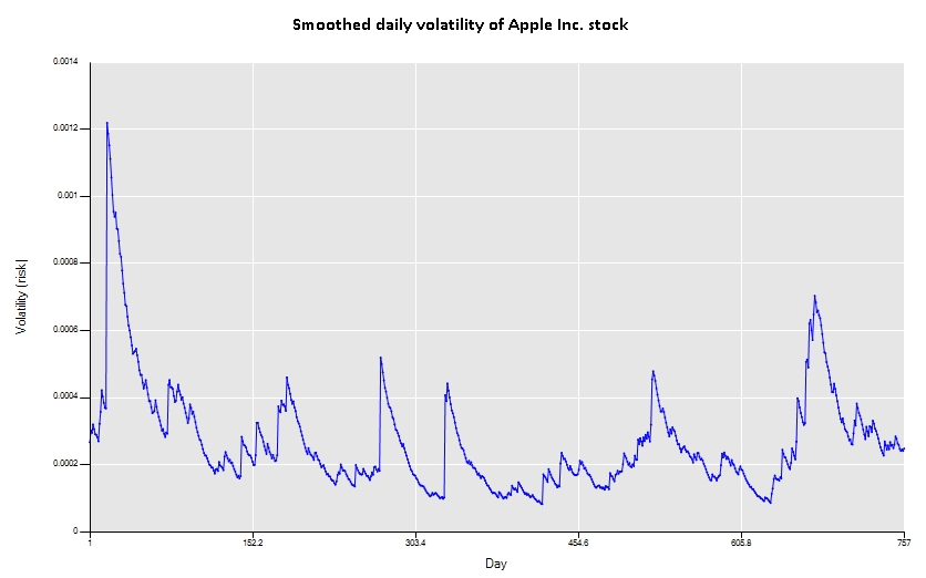
We need the following chain of transformations: 1º- Transform price to log returns, 2º- Square the returns to get a measure of an instantaneous volatility, 3º smooth the volatility using the exponential weighted moving average model.
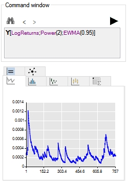
For the first transformation, we can use directly the “LogReturns” transformation or the pair 1st_Difference;Log. The second transformation can be done by the power(2) transformation or to be picky with volatility definition we can use the “Series-Mean_Squared” (the mean of logreturns is very close to zero for daily returns). Now, to smooth the results, we can apply an EWMA model with a decaying factor of 0.95, that is, use the transformation “EWMA(0.95)”. Putting it all together, we come to the following transformation string: Y[LogReturns;Power(2);EWMA(0.95)]. The screenshot of insertion box and the result is displayed below:


As a final remark, please note that when you have only one time series the explicitness of the operator Y[] is not necessary. Besides, the command window is not case sensitive. So, typing “Power” and “POWER” will lead to the same results.