
Learning Center
How to perform complex portfolio selection using utility functions?
The modern theory of portfolio selection generally is built on the assumption that an investor is concerned solely with the mean and variance of his portfolio. As pointed by Levy and Markowitz (1979), mean-variance portfolio selection is much more robust than commonly understood and can provide good approximations of the optimal portfolio even if the underlying model assumptions (i.e., elliptical distributions of returns and quadratic utility of wealth) do not hold. However, there are some plausible situations in which mean-variance analysis is not suitable, such as:
- The investor does care about higher moments of return distributions, such as the skewness.
- The model used by the investor for returns simulation is path dependent.
- There is a minimum return requirement that the investor considers to be very painful not to respect it.
- The attitude towards risk of an investor differs when he is evaluating gains or facing possible losses. This fact was endorsed by Kahneman and Tversky (1979) that proposed an accurate description of how decision makers behave when evaluating real-life investment choices which differ from the traditional view of the rational economic investor.
- The possibility of investing in non-linear assets (such as stocks options) is also being considered in the portfolio composition.
- The investor wants to evaluate how transaction costs affect his portfolio composition.
- The investor is designing an Asset and Liability Management Model that explicitly considers the possibility of rebalancing his portfolio over time.
SAFE TOOLBOXES® comes with many utility functions that can be very useful to help you find optimal portfolios in these situations. After giving a brief overview of what utility functions look like, we will provide you a complete example on how to use SAFE TOOLBOXES® to build a sophisticated portfolio selection.
What are utility functions and how to call them in SAFE TOOLBOXES®?
In short, utility functions are mathematical functions used to rank the investor’s preferences over many possible financial decisions and their potential outcomes.
A utility function u(w) that links the satisfaction that an investor receives from any specified level of wealth, w, may take many forms. However, it can be decomposed in some economic properties that will dictate the choices that the investor will make when evaluating financial alternatives. The properties are listed below:
- More wealth is preferred than less. Therefore, the first requirement placed on a utility function is that it has a positive first derivative (u’(w)>0).
- The investor's attitude towards risk. In this case, the investor can be averse to risk (u’’(w)<0), neutral towards risk(u’’(w)=0), or seeks risk (u’’(w)>0).
- The change in investor’s preferences with fluctuations in wealth. Defining the Absolute Risk Aversion – ARA(w) as -u’’(w)/u’(w), if an investor decreases the amount invested in risky assets as wealth increases, that investor is said to exhibit increasing absolute risk aversion, i.e., ARA’(w) >0.
- How the percentage of wealth invested in risky assets changes as wealth fluctuates. Defining the Relative Risk Aversion – RRA(w) as -w(u’’(w)/u’(w)), if the percentage invested in risky assets declines as wealth increases, that investor is said to exhibit increasing relative risk aversion, i.e., RRA’(w) >0
All SAFE TOOLBOXES®’ utility functions come with a parameter named “WealthOrReturnOrWealthFullReportString”. If you type “Wealth” you must enter a wealth value, w, to get the value of the utility function u(w). If you type “Return”, you can specify directly a return value, r, to get the utility function u(r): = u(w=1+r)-u(w=1). You can also type “WealthFullReport” to get a detailed report of the chosen utility function’s economics properties at the specified level of wealth.
The table below summarizes the utility functions available in SAFE TOOLBOXES®:
Function name |
Function formula |
sPortfolio_UtilityFunction_Exponential |
-exp(-a * w) |
sPortfolio_UtilityFunction_Power |
-w ^ (-a + 1) / (a - 1) |
sPortfolio_UtilityFunction_GeneralizedLog |
log(a + w) |
sPortfolio_UtilityFunction_Quadratic |
a * w ^ 2 + b * w + c |
sPortfolio_UtilityFunction_DoubleExponential |
a * exp(b * w) + c * exp(d * w) |
sPortfolio_UtilityFunction_LinearTimesExponential |
(a * w + b) * exp(c * w) |
sPortfolio_UtilityFunction_MixedPowerAndExponential |
-a * exp(-b * w) - 1 / w |
sPortfolio_UtilityFunction_QuadraticKinkedDownside |
w-1 / 2 * max(target - w,0) ^ 2 * q |
sPortfolio_UtilityFunction_LinearKinkedDownside |
w- max(target - w,0) *l |
sPortfolio_UtilityFunction_MixedQuadraticAndLinearKinkedDownside |
w-1 / 2 * max(target - w,0) ^ 2 * q- max(target - w,0) *l |
sPortfolio_UtilityFunction_PowerLinearKinkedDownside |
-LinearConst*max(target-w,0) - w ^ (-PowerConst+ 1) / (PowerConst - 1) |
sPortfolio_UtilityFunction_ProspectTheory |
MultUp* (target - w) ^ PowerUp , if w>=target, -MultDown(target - w) ^ PowerDown, if w<target |
Portfolio selection with utility functions
Performing portfolio selection using utility function follows a Simulation and Optimization approach. To illustrate the power of this method, let’s select a one-year portfolio based on the following data and assumptions:
- The list of available stocks to invest in are Exxon Mobil Corporation, Apple Inc., Microsoft Corporation, Wells Fargo & Company and Johnson & Johnson.
- The investor is also allowed to buy a put option on Apple stock with a strike price 5% higher than the stock is currently quoted. The put option costs 3% of the stock price and will expire after one year. The investor is also forbidden to spend more than 10% of his total wealth on put options.
- No parametric assumption of returns distribution is made. The portfolio must be chosen using the empirical distribution of returns, collected from January/2008 to December/2017.
- The investor’s preferences are represented by a power utility function (PowerConst=2) with an extra penalty (LinearConst=1) when the returns are below his target return of 3%.
- No short sales are allowed.
So, the steps required to perform our model are presented below:
Step 1: Build a Bootstrapping Simulation model.
Step 2: Get the result of your utility function for an arbitrary fixed decision.
Step 3: Compute the expectation of your utility function using the “Data Table” approach.
Step 1: Build a Bootstrapping Simulation model.
Bootstrapping is similar to Monte Carlo Simulation, but the simulated observations are selected from an empirical distribution instead of a parametrical one. To perform a Bootstrap Simulation just number the months to draw, from a uniform distribution, a sample month of returns. The spreadsheet below illustrates how it can be done in Microsoft Excel:
|
A |
B |
C |
D |
E |
F |
G |
H |
1 |
Example of a complex portfolio selection using utility functions |
|
|
|||||
2 |
|
|
|
|
|
|
|
|
3 |
|
1 |
2 |
3 |
4 |
5 |
6 |
|
4 |
Random month |
Apple Inc. |
Microsoft Corporation |
Exxon Mobil Corporation |
Wells Fargo & Company |
Johnson & Johnson |
Apple Inc. Put option |
|
5 |
119 |
1.02 |
1.01 |
1.00 |
1.01 |
1.00 |
<=1+VLOOKUP($A5,DataBase!$A:$F,F$3+1,FALSE) |
|
6 |
49 |
1.13 |
1.14 |
0.99 |
1.06 |
1.01 |
|
|
7 |
28 |
1.11 |
1.04 |
1.01 |
1.06 |
0.99 |
|
|
8 |
108 |
1.05 |
1.04 |
1.04 |
1.05 |
1.04 |
|
|
9 |
16 |
1.20 |
1.10 |
0.98 |
1.41 |
1.00 |
|
|
10 |
93 |
0.98 |
1.02 |
1.00 |
0.96 |
1.00 |
|
|
11 |
29 |
0.98 |
0.84 |
0.89 |
0.87 |
0.91 |
|
|
12 |
10 |
0.95 |
0.84 |
0.95 |
0.91 |
0.89 |
|
|
13 |
28 |
1.11 |
1.04 |
1.01 |
1.06 |
0.99 |
|
|
14 |
107 |
0.97 |
1.01 |
1.05 |
1.15 |
0.96 |
|
|
15 |
=RANDBETWEEN(1,120) |
1.10 |
1.02 |
0.94 |
1.03 |
1.00 |
|
|
16 |
45 |
0.99 |
0.94 |
0.99 |
0.93 |
0.98 |
|
|
17 |
|
|
|
|
|
|
|
|
18 |
Overall return |
73.1% |
=PRODUCT(C5:C16)-1 |
-15.1% |
46.7% |
-23.4% |
-100.0% |
<=MAX(5%-B18,0)/3%-1 |
19 |
|
|
|
|
|
|
|
|
Step 2: Get the result of your utility function for an arbitrary fixed decision.
Once you get your sample year returns for each stock, you can compute the overall portfolio return and its correspondent utility using the formulas as shown in the below spreadsheet:
|
A |
B |
C |
D |
E |
F |
G |
H |
17 |
|
|
|
|
|
|
|
|
18 |
Overall return |
73.1% |
0.0% |
-15.1% |
46.7% |
-23.4% |
-100.0% |
<=MAX(5%-B18,0)/3%-1 |
19 |
|
|
|
|
|
|
|
|
20 |
Assets proportion |
20.0% |
20.0% |
20.0% |
20.0% |
20.0% |
0.0% |
<=1-SUM(B20:F20) |
21 |
|
|
|
|
|
|
|
|
22 |
Portfolio return |
16.27% |
<=SUMPRODUCT(B18:G18,B20:G20) |
|
|
|
|
|
23 |
Target return |
3% |
|
|
|
|
|
|
24 |
Power constant |
2 |
|
|
|
|
|
|
25 |
Linear constant |
1 |
|
|
|
|
|
|
26 |
Utility of return |
0.1399 |
<=sPortfolio_UtilityFunction_PowerLinearKinkedDownside(B22,"Return",B23,B24,B25) |
|
||||
27 |
|
|
|
|
|
|
|
|
Step 3: Compute the expectation of your utility function using the “Data Table” approach.
To get the expectation of your utility function based on 1,000 portfolio returns samples, first create a table as follows: enter a sequence from 1 to 1000 in cells A32:A1031 and put the formula "=B26" in cell B31.
Then, select the range A31:B1031, go to Data > What-if analysis > Data table… and type B29 in the “Column input cell” field. After doing that, you can compute the expected value of your utility function using the Excel’s average formula in cell B28. The resulting spreadsheet is the following:
|
A |
B |
C |
D |
E |
F |
G |
H |
26 |
Utility of return |
0.1399 |
<=sPortfolio_UtilityFunction_PowerLinearKinkedDownside(B22,"Return",B23,B24,B25) |
|
||||
27 |
|
|
|
|
|
|
|
|
28 |
Expected utility of return |
0.0871 |
<=AVERAGE(B32:B1031) |
|
|
|
|
|
29 |
Random number to force recalculation |
0.95 |
<=RAND() |
|
|
|
|
|
30 |
|
|
|
|
|
|
|
|
31 |
|
0.1751 |
<=B26 |
|
|
|
|
|
32 |
1 |
0.2600 |
|
|
|
|
|
|
33 |
2 |
-0.0430 |
|
|
|
|
|
|
34 |
3 |
0.1210 |
|
|
|
|
|
|
35 |
4 |
0.2955 |
|
|
|
|
|
|
36 |
5 |
0.2663 |
|
|
|
|
|
|
… |
… |
… |
… |
… |
… |
… |
… |
… |
1028 |
996 |
0.1220 |
|
|
|
|
|
|
1029 |
997 |
0.1676 |
|
|
|
|
|
|
1030 |
998 |
0.1771 |
|
|
|
|
|
|
1031 |
999 |
-0.5780 |
|
|
|
|
|
|
1032 |
1000 |
0.2554 |
|
|
|
|
|
|
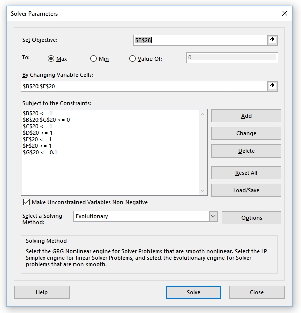
Step 4: Find the portfolio that maximizes the expectation of your utility function using Microsoft Solver.
Finally, Microsoft Solver can be used to get the asset allocation that maximizes the expected value of the utility function. As the objective function is not smooth, you may have to use the “Evolutionary Solver” to look for a good solution for your maximization problem. The screenshot below illustrate a possible solver configuration:
In our example, after solving the problem, the best portfolio found was the following:
|
A |
B |
C |
D |
E |
F |
G |
H |
19 |
|
|
|
|
|
|
|
|
20 |
Assets proportion |
69.4% |
3.6% |
7.7% |
8.5% |
7.6% |
3.2% |
<=1-SUM(B20:F20) |
21 |
|
|
|
|
|
|
|
|
22 |
Portfolio return |
40.80% |
<=SUMPRODUCT(B18:G18,B20:G20) |
|
|
|
|
|
23 |
Target return |
3% |
|
|
|
|
|
|
24 |
Power constant |
2 |
|
|
|
|
|
|
25 |
Linear constant |
1 |
|
|
|
|
|
|
26 |
Utility of return |
0.2897 |
<=sPortfolio_UtilityFunction_PowerLinearKinkedDownside(B22,"Return",B23,B24,B25) |
|
||||
27 |
|
|
|
|
|
|
|
|
28 |
Expected utility of return |
0.1846 |
<=AVERAGE(B32:B1031) |
|
|
|
|
|
Please note that the “Evolutionary Solver” and the “Data Table” are very time-consuming methods and it could take a while until you get all the optimization done. Besides that, as the procedures are based on non-deterministic approaches the results can vary from one simulation to another.
References
H. Levy and H. Markowitz. 1979. “Approximating Expected Utility by a Function of Mean and Variance,” American Economic Review (June).
Kahneman, Daniel; Tversky, Amos (1979). “Prospect Theory: An Analysis of Decision under Risk". Econometrica. 47 (2): 263.